Oscillation

This activity is aimed at upper-secondary students who are not afraid of linear combinations, roots, exponential functions and logarithms. They are also interested in “guessing” physical laws from data without a background in physics.

Spring pendulum

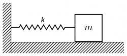
We will be dealing with a horizontal spring pendulum. We have an object or a weight with mass m lying on a cart or a smooth frictionless surface. The weight is attached to a wall with a coil spring of spring constant k. We pull the weight from its equilibrium position by a displacement d and then release it. What will be the oscillating time of the object?

Let’s start by reflecting on the problem. How do the mass of the weight, the spring constant, and the initial displacement from equilibrium affect the oscillating time of the spring pendulum? Do they increase it, decrease it, or have no influence on it? (We will discover the correct answers together, or you can find them in the conclusion.)

• What will happen to the oscillating time if we use a weight with a heavier mass?
• What if instead of a weight we replace the spring with a stiffer spring with a higher coefficient?
• Will the oscillating time be greater if the object is pulled further away from the equilibrium position?

It would be convenient to describe the physical phenomenon using existing knowledge of physics to derive an equation for the oscillation time. But we will approach the problem differently. We will try to determine an equation from experiments that fits the measured data as closely as possible, and finally see how successful we have been.

Data

We have prepared two datasets. The first uses only one spring and the second uses different springs. Both could have been obtained by performing experiments, but for the purpose of this exercise we preferred to generate the data randomly according to known physical laws, plus a little random “measurement” error. The individual measurements are described by the weight mass m [kg], the weight coefficient k [N/m], the displacement d [m] and the oscillating time t [s].

One spring

Let’s start with an easier problem, where we have the same spring all the time with coefficient k = 20 N/m. In the scatter plot we can see the attribute dependencies that will help us in further modelling. The offset does not tell us much about the oscillating time (bottom figure, left hand side), but the mass tells us much more (bottom figure, right hand side). The heavier the mass, the larger the oscillating time. However, this relationship is not completely linear, so that twice the mass means twice the oscillating time.

We will try to model the relationship between mass and oscillating time as best we can with the equation of the line or linear equation t = a₁ + a₂ * m. We want to find the numbers a₁ and a₂ so that the line fits the data as closely as possible. We will use the Polynomial Regression widget from the Orange Educational add-on. This allows you to find approximations with higher degree polynomials, but we will be interested in an approximation with a linear function that is a first degree polynomial.

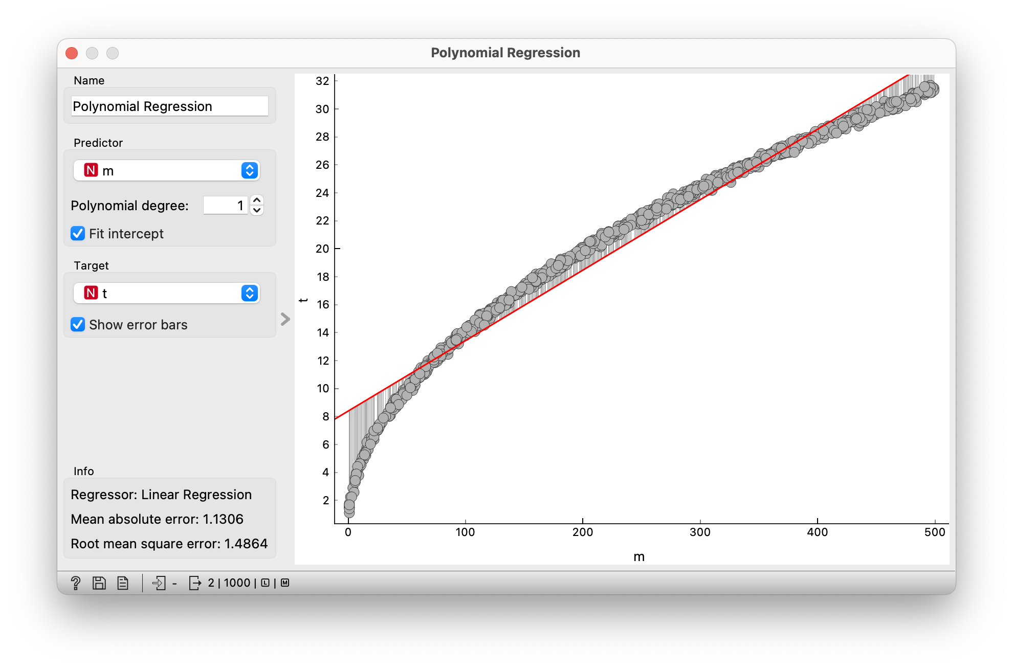
In the figure, the best approximation is shown by the red line and the deviations of the points from the straight line are indicated by the vertical lines. One measure of the deviation is the RMSE (Root mean square error), which in our case has a value of 1.49. Using the data table we can also see the actual coefficients of the line (in our case a₁ = 8.39 and a₂ = 0.05). The equation of the line is therefore t = 8.39 + 0.05 * m.

We see that the dependence looks similar to the root function, so we will add a new attribute equal to the root of the weight mass, so Km = √(m). If we now use polynomial regression to model the oscillating time t as a function of the new attribute Km, we will be much more successful. This leads to the equation t = 0.00 + 1.41 *Km.

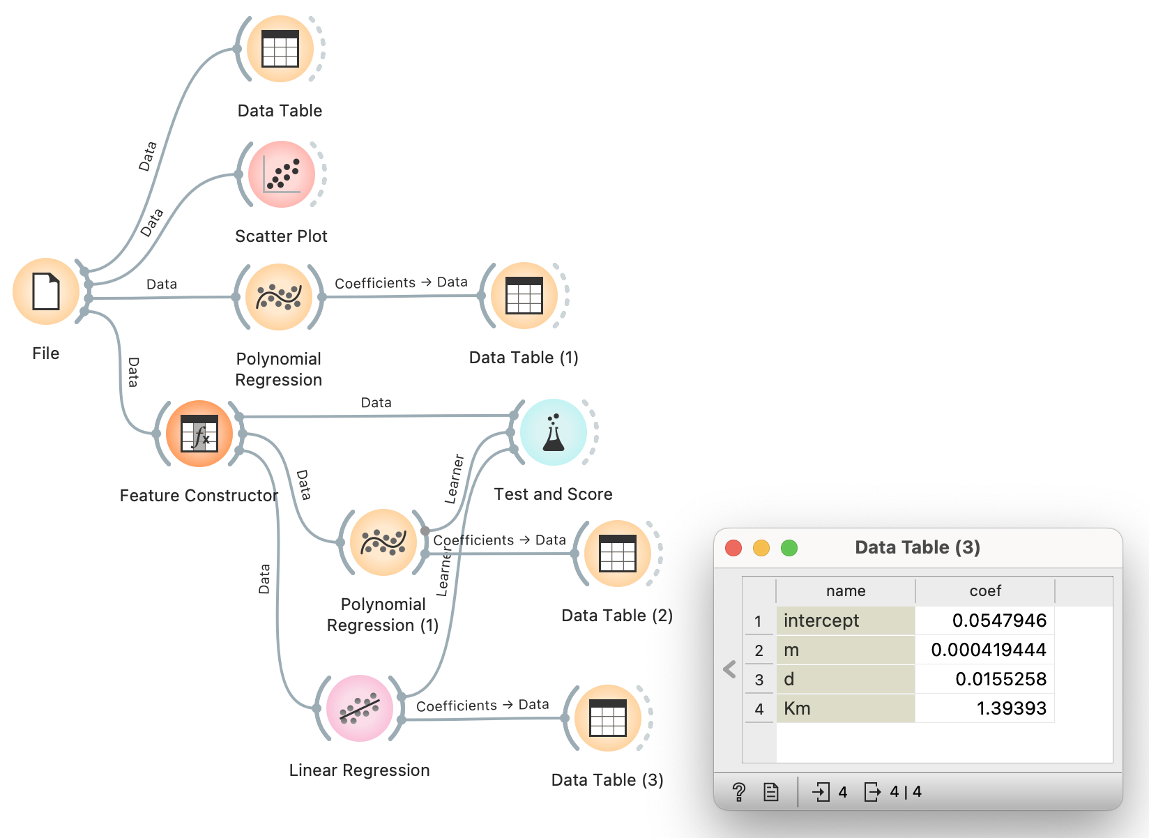
So far we have been looking for the dependence of the oscillating time on a single attribute, but we have several attributes available. But what if we considered several attributes at once and found the coefficients of a (a₀, a_Km, a_m, a_d) that would model the oscillating time as best as possible with the equation t = a₀ + a_Km * Km + a_m * m + a_d * d.

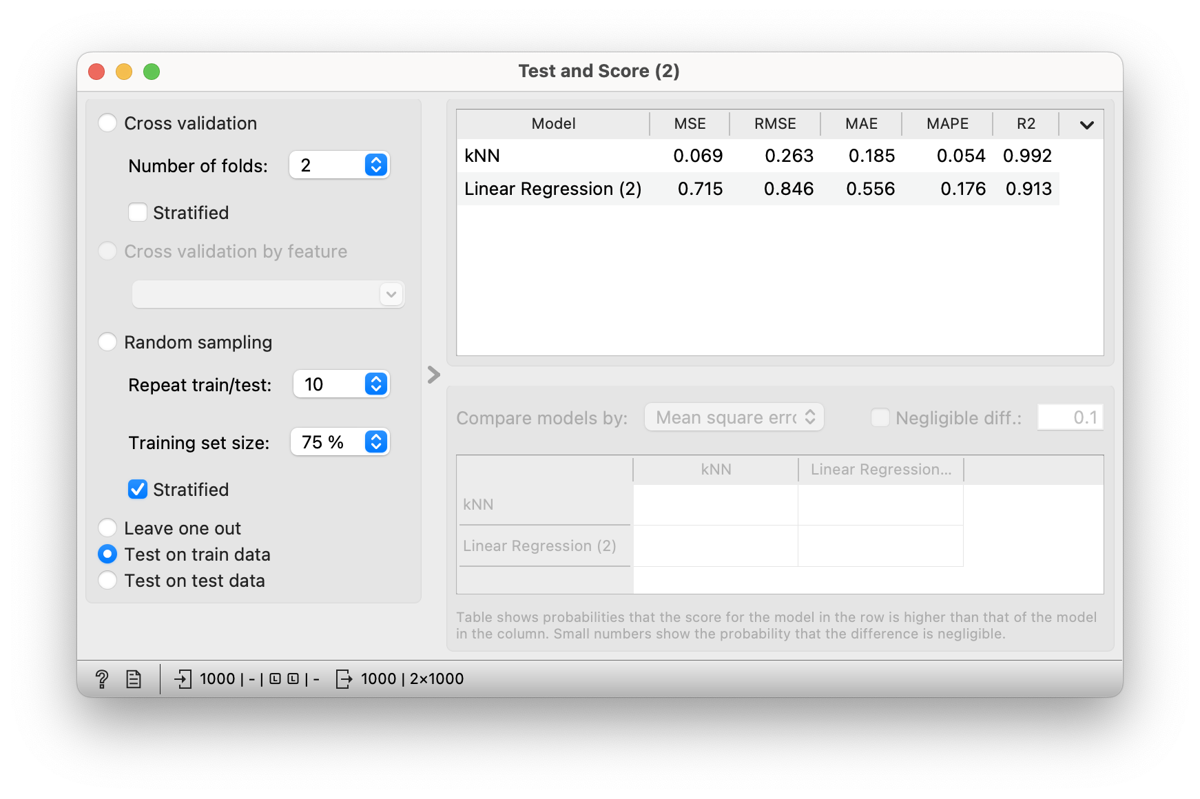
This is the purpose of linear regression, which reveals the equation t = 0.05 + 1.39 * Km + 0.00 * m + 0.02 * d. If we compare the performance (RMSE) of a polynomial regression and a linear regression using the Test and Score widget, we will see that they have practically the same performance. Therefore, we will ignore the small coefficients without much harm. Thus, we now have the equation t = 1.39 * √m.

Different springs

From the previous result, we can conclude that the oscillation time is independent of the displacement d, so it will not be used in the following. The data can be subjected to linear regression and the initial deviation RMSE = 1.415 is obtained, which we will try to reduce. If we could ideally model the oscillation time, the RMSE would be 0, but this will not be possible due to the measurement errors in our data.

We also know that the root of the mass worked well, so let’s add the root of the spring coefficient and look at the data in the scatter plot. This time we are looking at the dependence of time on two variables Km = √m and Kk = √k. In the diagram, we will therefore represent time by colour. It can be seen that the oscillation time is larger for heavier masses and for smaller weight coefficients. However, we cannot conclude much more from this.

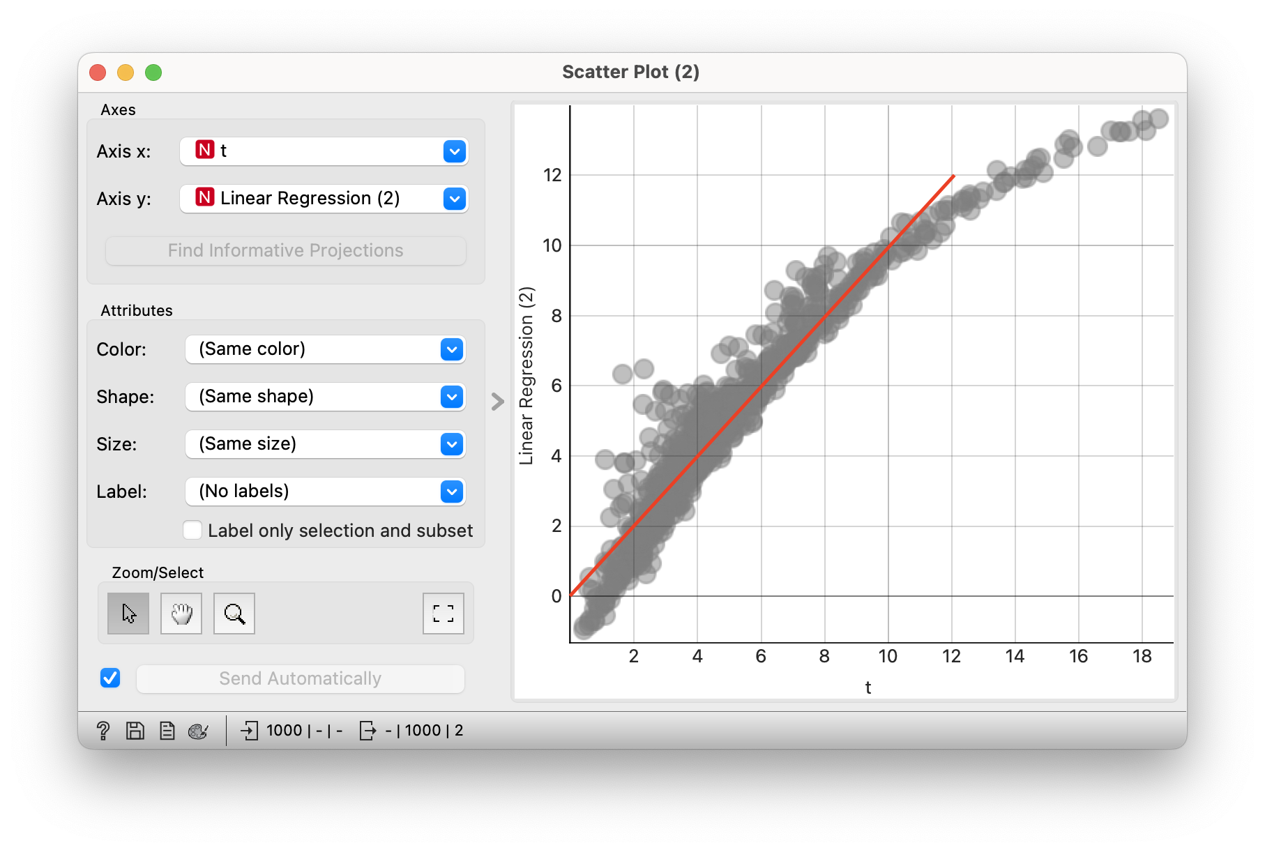
Let’s now give all the attributes to the linear regression to find the coefficients to best model time and check its performance. The equation t = 13.11 + 0.00 * m + 0.09 * k + 0.75 * Km - 2.31 * Kk gives RMSE = 0.846, which is already an improvement on our first attempt (RMSE = 1.415). The addition of roots therefore helps the modelling. In the scatter plot, we can compare the actual oscillating time and the predicted value. If our predictions were very accurate, we would expect to see all points on the diagonal (marked red in the figure). However, we notice that this is not quite the case. Especially for larger oscillating times, the model misses quite a lot. On the other hand, at small oscillating times, some of the predictions are even negative!

If we are only interested in predicting the oscillating times, we can use a simple nearest-neighbour prediction approach. For the given attributes (mass and weighting coefficient), we find some of the most similar examples ( for example 5) and predict their average value. This approach is much more accurate, but it does not help us in the interpretation. From such a model we cannot infer anything new about the physical process from the data.

Logarithms

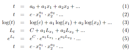
We know from experience that the equation we are looking for is probably not a linear combination of the form (1), where x₁, x₂, … naši atributiare our attributes, but will be some product of potentials of the form (2), where we are looking for the coefficients c, a₁, a₂, … We have linear regression, which is able to find the coefficients in an equation of the first form, but we are interested in the coefficients in an equation of the second form. We can use logarithms to help us do this. Let us logarithm both sides of equation (2) to obtain an equation of the form (3) and write it with new variables (4) representing the logarithms of the attributes. The coefficients in this new equation can then be found by linear regression. So we have a tool that is able to model the logarithms of the attributes we are working with. Using linear regression, we calculate the coefficients of C, a₁, a₂, … in equation (4), and then we have to convert it all back. We do this using the exponential function (5) and obtain the final form (6). (Note: c = e^C)

Use the Feature Constructor widget to construct new attributes that are logarithms of the existing ones, and then use the Select Columns widget to select only the new attributes, so that you don’t have a mixture of logarithmic and non-logarithmic attributes. Using linear regression, we can now achieve an RMSE = 0.065, which is very close to zero, representing an almost perfect fit of the model to the actual values. However, this RMSE value should not be compared with the previous ones! We are now modelling the logarithms of the values. Using the coefficients found by the linear regression, we get the equation t = e^1.838 * m^0.502 * k^-0.503.

We can now create a new variable x to represent our prediction using the equation we discovered earlier. For the purpose of checking the accuracy of the prediction, let’s select only our predictor variable from the attributes and use polynomial regression to check its usefulness. We obtain RMSE = 0.199, which is much better than our previous experiments (1.415 and 0.846). Looking at the polynomial regression, it makes practically no change to our predictor variable.

In solving our problem, we have put together quite an impressive workflow.

Conclusion

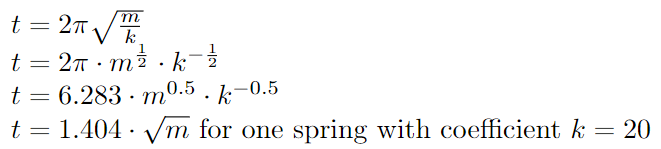
What do those who know physics say about a spring pendulum? Below is the correct equation of the oscillating time for a spring pendulum and its alternative forms for comparison with the equations discovered. If we round our discovery and simplify it a little, we get t = 6.28 * √m / √k. We can see that our approximations were very close to the true values despite the measurement errors in the data.

Let’s look at the answers to the initial questions, which should now be clear:

• Increasing the mass increases the oscillating time. It takes longer to move or swing (oscillate) an object with more mass.
• Increasing the spring coefficient decreases the swing time. The stiffer the spring, the faster the weight swings back and forth.
• The initial displacement has no effect on the swing time. At least not in the case of an ideal spring with a coefficient that does not depend on the displacement.

The same experiment could be carried out for a vertically fixed spring pendulum, as the same properties apply, except that the initial equilibrium position is slightly different due to gravity.